ADI:Enhancing the Performance of Pedometers Using a Single Accelerometer

ApplICation note AN-602 examined the use of an Analog Devices accelerometer to make a simple but relatively accurate pedometer. Since that time, newer devices have been introduced that allow the use of accelerometers in more cost-sensitive applications. Thus, applications such as pedometers are finding themselves in many consumer devices such as cellular handsets.

Given this trend, a closer examination was made of pedometers using a single accelerometer. The AN-602 technique was implemented in an attempt to duplicate its results. Though the algorithm performed well, the same accuracy was not duplicated. In particular, there was greater variation than expected from person to person, as well as when one person used a different pace and stride length. This led to an investigation of potential improvements to the algorithm.

Tests were done using the ADuC7020 precision analog microcontroller with ARM7 core and two different pedometer test boards: one with a 2-axis ADXL323 accelerometer and one with a 3-axis ADXL330 accelerometer. The first used ADuC7020 and ADXL323 evaluation boards with an added 16 × 2 LCD display. The second used a custom board.

AN-602 Method

The technique used in AN-602is based on the principle that the vertical “bounce” in one’s step is directly correlated to the stride length, as shown in Figure 1.

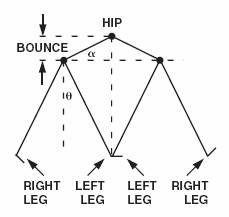
The angles α and θ are equal, so the stride can be shown to be a multiple of the maximum vertical displacement. Given the same angles, the vertical displacement would be greater or smaller for taller or shorter people, thus accounting for differences in leg length.

Unfortunately, the accelerometer measures changes in acceleration rather than displacement. The acceleration must be converted to distance before it can be used. In the AN-602 setup, limited computing power required that a simple formula be used to approximate the double integral needed to convert acceleration into distance.

With plenty of processing power available in the ADuC7020, this experiment attempts to directly calculate the discrete integrals. A simple method was chosen to do this. After each step was determined, all of the acceleration samples within that step were added to get a set of velocity samples. The velocity samples for each step were normalized such that the final sample was zero. They were then added together to get a value for the displacement.

Initially, this technique looked promising, as measured distances were relatively consistent for one subject walking a course multiple times. Unfortunately, the person-to-person variance was exacerbated, as was the variance for one subject at different paces. This led to an investigation of whether the problem is with the model itself.

Understanding the Model

This model has two primary assumptions: that the foot is actually a single point (or a ball), and that the impact of each foot on the ground is perfectly elastic. Neither of these assumptions is the case, however. based on these experiments, it is safe to say that the differences between these assumptions and reality explain much of the encountered variations.

To understand this, it helps to look at the measured acceleration over several steps, as shown in Figure 2. Different sources of “spring” in one’s step are shown on the data.

Figure 2 demonstrates the problems encountered with trying to accurately translate measured acceleration into distance. Methods that use the peak-to-peak change—and even those that integrate the data—run into trouble with data like this. The cause of this difficulty is the variation from one measurement to another in spring of different people’s steps, or in the steps of one person using different paces.

Figure 3 shows the same subject with a longer and faster stride. The peak-to-peak acceleration difference is larger, and the various spring points look different. The amount of “spring” data versus “real” data is different than in Figure 2. But the algorithm only sees a set of acceleration measurements, and has no idea of the context of those measurements. The problem, therefore, is to remove the effect of the spring in a subject’s step without removing useful data.

There are important differences between the two plots: In Figure 3, the bottom of the curve for each step is slightly narrower than that of Figure 2, and the tops of the curves are more consistent, with fewer distinctive peaks. These differences result in a higher average value compared to the minimum and maximum sample values.

For comparison purposes, Figure 4 shows a data plot for a different individual. The stride length is very similar to that of the subject in Figure 2. The data itself looks very different, however.

This subject’s stride has a great deal more spring in it than that shown in Figure 2, but both sets of data represent roughly the same distance walked. Calculating distance solely on the peak values will thus give widely varying results. Using a simple double integration suffers from the same problem.

Solving the problem of spring

All efforts to come up with a decent solution to this problem using straightforward calculations had the same problems, leading to a series of failed attempts to normalize the data in a way that eliminated the spring. The main reason seemed to be that they required some knowledge of the context of the data but, in actual use, the system has no idea what is going on outside. All it has are data points. Our solution needs to be able to operate on the data without context.

During an episode of frustration, a possible solution to this problem presented itself. As noted earlier, the data changed when going from a slower to faster pace, but less apparent variation due to the spring occurred with a longer, quicker stride. The result was a higher average with respect to the data minima and maxima. But would this hold up with new data?

Visually, it’s difficult to be sure of this, given the amount of bounce in the steps shown in Figure 4. But calculations showed that the average-versus-peak values are very similar to those in Figure 2. So, a candidate for a simple algorithm to determine the distance walked is:

This calculation is done for each step, as determined by a different step-finding algorithm. The step-finding algorithm uses an 8-point moving average to smooth the data. It searches for a maximum peak, followed by a minimum. A step is counted when the moving average crosses the zero point, which is the overall average for the step. The data used in the distance algorithm takes into account the 4-point latency of the moving average.

This simple solution held up well for the first subject over various stride lengths. It also did reasonably well with additional subjects. But some subjects produced distances that varied as much as 10% from the average measured distance for the group. This wasn’t within the ±7.5% error band that was targeted for an uncalibrated measurement. Another solution was needed.

Still, the ratio used in the last test seemed to reflect differences in the spring of different subjects’ steps. It made sense to try combining the two methods we’ve examined here. Going back to the original idea of using a double integral, a calculation was made using this ratio as a correction factor to remove the spring data. The resulting formula is:

Where:
d is the distance calculated
k is a constant multiplier
max is the maximum acceleration measured within this step
min is the minimum acceleration measured within this step
avg is the average acceleration value for the step
accel represents all measured acceleration values for the step

This algorithm held up well for a variety of subjects and paces, varying by about +6%/–4%. The algorithm lends itself to easy calibration for a specific individual and pace by adjusting the multiplier k. The code can also perform an average on the stride length to smooth out step-to-step variation. The results mentioned here did not include the use of this averaging.

In this experiment only the X- and Y-axes were used. A 3-axis accelerometer was chosen for flexibility, in case all three axes were needed. Two axes were found to be adequate for the task, so an ADXL323 could be used in place of the ADXL330. The same layout can be used for both since the pin configuration is identical excepting the Z-axis output.

This experiment focused on achieving good results for the pedometer’s distance measurement.  The step-counting algorithm was evaluated only enough to ensure that it worked well while walking or running. Over hundreds of walking or running steps, the measured number of steps fell within one or two steps of the actual number. Unfortunately, however, this simple algorithm can be fooled by non-walking motion. The time-window function described in AN-602 can be used to minimize miscounts by ignoring false steps that occur outside the expected time window, while retaining the ability to adapt when the user changes pace.

Summary

This note represents the results of a single set of experiments attempting to gain decent performance from a simple pedometer that uses a single accelerometer. Some of the barriers to gaining that performance have been discussed. The final results met the stated accuracy goals, with the added possibility of improved accuracy with calibration. While greater accuracy can be obtained with a more complex system (using multiple accelerometers, for instance), the algorithm provided here should be an excellent starting point for simple, low-cost applications.