

Making accurate high-speed time-domain measurements can be challenging, but finding information that will help improve one’s techniques shouldn’t be. Understanding the basICs of oscilloscopes and probes is always helpful, but a few extra tricks of the trade and some good old-fashioned commonsense engineering can be employed to help yield quick and accurate results. The following are some tips and techniques I’ve accumulated over the past 25 years. Incorporating even a few of these into your measurement kit could help improve your results.
Simply grabbing a scope off the shelf and a probe from the drawer won’t do for high-speed measurements. When choosing the right scope and probe for high-speed measurement, first consider: signal amplitude, source impedance, rise time, and bandwidth.
Selecting Oscilloscopes and Probes
There are hundreds of oscilloscopes available, ranging from very simple portable models to dedicated rack-mount digital storage scopes that can cost hundreds of thousands of dollars (some high-end probes alone can cost upwards of $10,000). The variety of probes that accompany these scopes is also quite impressive, including passive, active, current-measuring, optical, high-voltage, and differential types. It is beyond the scope of this article to provide a complete and thorough description of each and every scope and probe category available, so we will focus on scopes for high-speed voltage measurements utilizing passive probes.
The scopes and probes discussed here are used to measure signals characterized by wide bandwidths and short rise times. Besides these specifications, one needs to know about the circuit’s sensitivities to loading—resistive, capacitive, and inductive. Fast rise times can become distorted when high-capacitance probes are used; and in some applications the circuit may not tolerate the presence of the probe at all (for example, some high-speed amplifiers will ring when capacitance is placed on their output). Knowing the circuit limitations and expectations will help you to select the right combination of scope and probe and the best techniques for using them.
To start, the signal bandwidth and rise time will limit the scope choices. A general guideline is that scope and probe bandwidth should be at least three to five times the bandwidth of the signal being measured.
Bandwidth
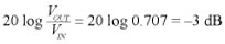
Whether the signal being measured occurs in an analog or a digital circuit, the scope needs to have enough bandwidth to faithfully reproduce the signal. For analog measurements, the highest frequency being measured will determine the scope bandwidth. For digital measurements, it is usually the rise time—not the repetition rate—that determines the required bandwidth. The bandwidth of the oscilloscope is characterized by its –3 dB frequency, the point at which a sine wave’s displayed amplitude has dropped to 70.7% of the input amplitude, that is
 | (1) |
It is important to ensure that the oscilloscope has sufficient bandwidth to minimize errors. Measurements should never be made at frequencies near the oscilloscope’s –3 dB bandwidth, as this would introduce an automatic 30% amplitude error in a sine-wave measurement. Figure 1 is a convenient plot showing typical derating of amplitude accuracy vs. the ratio of the highest frequency being measured to scope bandwidth.
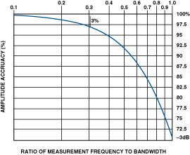
For example, a 300 MHz scope will have up to 30% error at 300 MHz. In order to keep errors below the 3% mark, the maximum signal bandwidth that can be measured is about 0.3 × 300 MHz, or 90 MHz. Stated another way, to accurately measure a 100 MHz signal (<3% error), you need at least 300 MHz of bandwidth. The plot in Figure 1 illustrates a key point: to keep amplitude errors reasonable, the bandwidth of the scope and probe combination should be at least three to five times the bandwidth of the signal being measured. For amplitude errors to be less than 1%, the scope bandwidth needs to be at least five times the signal bandwidth.
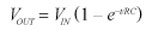
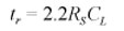
For digital circuits, rise time is of particular interest. To ensure that the scope will faithfully reproduce rise times, the expected or anticipated rise time can be used to determine the bandwidth requirements of the scope. The relationship assumes the circuit responds like a single-pole, low-pass RC network, as shown in Figure 2.
In response to an applied voltage step, the output voltage can be calculated using Equation 2.
 | (2) |
The rise time in response to a step is defined as the time it takes for the output to go from 10% to 90% of the step amplitude. Using Equation 2, the 10% point of a pulse is 0.1 RC and the 90% point is 2.3 RC. The difference between them is 2.2 RC. Since the –3 dB bandwidth, f, is equal to 1/(2πRC), and the rise time, tr, is 2.2 RC,
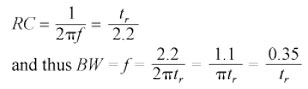 | (3) |
So, with a single-pole probe response, one can use Equation 3 to solve for a signal’s equivalent bandwidth, knowing the rise time. For example, if a signal’s rise time is 2 ns, the equivalent bandwidth is 175 MHz.
 | (4) |
To keep errors to 3%, the scope-plus-probe bandwidth should be at least three times faster than the signal being measured. Therefore a 600 MHz scope should be used to accurately measure a 2 ns rise time.
Probe Anatomy
Given their simplicity, probes are quite remarkable devices. A probe consists of a probe tip (which contains a parallel RC network), a length of shielded wire, a compensation network, and a ground clip. The probe’s foremost requirement is to provide a noninvasive interface between the scope and the circuit—disturbing the circuit as little as possible, while allowing the scope to render a near-perfect representation of the signal being measured.
Probes got their start back in the days of vacuum tubes. For measurements at the grids and plates, a high impedance was required to minimize loading of the signal node. This principle is still important today. A high-impedance probe will not significantly load the circuit, thus providing an accurate picture of what is truly going on at the measurement node.
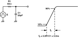
In my experience in the lab, the most commonly used probes are 10× and 1× passive probes; 10× active FET probes are a close second. The 10× passive probe attenuates the signal by a factor of 10. It has 10M ohm input impedance and 10 pF typical tip capacitance. The 1× probe, with no attenuation, measures the signal directly. It has 1M ohm input impedance, and tip capacitance as high as 100 pF. Figure 3 shows a typical schematic for a 10×, 10M ohm probe.
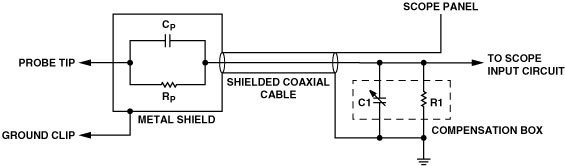
RP (9M ohm) and Cp are in the probe tip, R1 is the scope input resistance, and C1 combines the scope input capacitance and the capacitance in the compensation box of the probe. For accurate measurements, the two RC time constants (RpCp and R1C1) must be equal; imbalances can introduce errors in both rise time and amplitude. Thus, it is extremely important to always calibrate the scope and probe prior to making measurements.
Calibration
One of the first things that should be done after acquiring a working scope and probe is to calibrate the probe to ensure that its internal RC time constants are matched. Too often this step is skipped, as it is seen as unnecessary.
Figure 4 shows how to properly connect the probe to the probe compensation output of the scope. Calibration is accomplished by turning the adjustment screw on the compensation box with a nonmagnetic adjustment tool until a flat response is achieved.
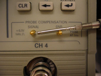
Figure 5 shows the waveforms produced by a probe that is undercompensated, overcompensated, and properly compensated.
Note how an undercompensated or overcompensated probe can introduce significant errors in rise time and amplitude measurements. Some scopes have built-in calibrations. If your scope has one, make sure you run it before making measurements.
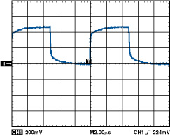
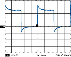
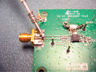
Figure 5. Probe compensation: a) undercompensated. b) overcompensated. c) properly compensated.
Ground Clips and High-Speed Measurements
Their inherent parasitic inductance makes ground clips and practical high-speed measurements mutually exclusive. Figure 6 shows a schematic representation of a scope probe with a ground clip. The probe LC combination forms a series resonant circuit—and resonant circuits are the basis of oscillators.
This added inductance is not a desirable feature, because the series-LC combination can add significant overshoot and ringing to an otherwise clean waveform. This ringing and overshoot often go unnoticed due to limited bandwidth of a scope. For example, if a signal containing a 200 MHz oscillation is measured with a 100 MHz scope, the ringing will not be visible, and the signal will be highly attenuated due to the limited bandwidth. Remember that, for a 100 MHz scope, Figure 1 showed 3 dB of attenuation at 100 MHz, with a continuing roll-off of 6 dB per octave. So the 200 MHz parasitic ringing will be down nearly 9 dB, a reduction to almost 35% of the original amplitude, making it difficult to see. With higher-speed measurements and wider-bandwidth scopes, however, the influence of ground clips is clearly visible.
The frequency of the ringing introduced by the ground clip can be approximated by calculating the series inductance of the ground clip using Equation 5. L is the inductance in nanohenrys, l is the length of the wire in inches, and d is the diameter of the wire in inches.
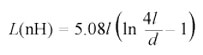 | (5) |
The result of Equation 5 can then be inserted into Equation 6 to calculate the resonant frequency, f (Hz). L is the inductance of the ground clip in henrys and C is the total capacitance (farads) at the node being probed—the probe capacitance plus any parasitic capacitance.
 | (6) |
Let’s look at a few examples using different lengths of ground clips. In the first example, an 11 pF probe is used with a 6.5 inch ground clip to measure a fast-rising pulse edge. The result is shown in Figure 7. The pulse response at first glance looks clean, but upon closer inspection, a very low-level 100 MHz damped oscillation can be seen.
Let’s substitute the physical features of the probe in Equations 5 and 6 to check if this 100 MHz oscillation is caused by the ground lead. The ground clip length is 6.5 inches and the diameter of the wire is 0.03 inches; this yields an inductance of 190 nH. Plugging this value into Equation 6, along with C = 13 pF (11 pF from the scope probe and 2 pF of stray capacitance) yields about 101 MHz. This good correlation with the observed frequency allows us to conclude that the 6.5 inch ground clip is the cause of the low-level oscillation.
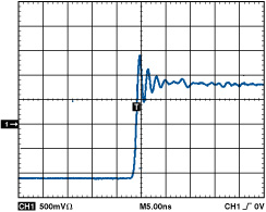
Now consider a more extreme case, where a faster signal, with a 2 ns rise time, is applied. This is typically found on many high-speed PC boards. Using a TDS2000-series scope, Figure 8a shows that there is significant overshoot and prolonged ringing. The reason is that the faster rise time of 2 ns, with its bandwidth equivalent of 175 MHz, has more than enough energy to stimulate the 100 MHz series LC of the probe lead to ring. The overshoot and ringing is approximately 50% peak to peak. Such effects from typical grounds are clearly visible and are totally unacceptable in high speed measurements.
By eliminating the ground lead, the response to the applied input signal is shown with much better fidelity (Figure 8b).
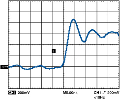
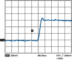
Figure 8. a) Response to step with 2 ns rise time with 6.5 inch ground clip. b) Step response with no ground lead.
Readying a Probe for High-Speed Measurements
In order to obtain meaningful scope plots we need to rid the circuit of the ground clip and dismantle the probe. That’s right, take that perfectly good probe apart! The first thing to discard is the press-on probe-tip adapter. Next, unscrew the plastic sleeve that surrounds the probe tip.
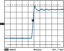
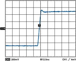
Figure 9. a) Probe right out of the box. b) Probe ready for high-speed measurements. c) Measurement with unmodified probe. d) Measurement with high-speed-ready probe.
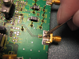
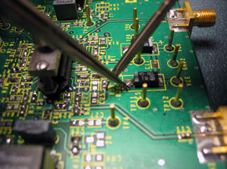
Figure 10. Ground methods for stripped-down scope probe.
Next to go is the ground clip. Figure 9 shows the before (a) and after (b) transformation of the scope probe. Figure 9c shows a measurement of a pulse generator’s rising edge, using a 6 inch ground clip; and (d) shows the same measurement with the probe configured for high-speed measurements, as shown in 9b. The results, like those of Figure 8, can be dramatic. Next, the simplified stripped down probe needs to be calibrated (see Figure 4). once calibrated, the probe is ready to use. Simply go to a test point and pick up a local ground on the outer metal shield of the probe. The trick is to pick up the ground connection right at the scope probe shield. This eliminates any of the series inductance introduced by using the supplied probe ground clip. Figure 10a shows the proper probing technique for using the streamlined probe. If ground can’t be conveniently contacted, use a pair of metal tweezers, a small screwdriver, or even a paper clip to pick up the ground connection, as shown in Figure 10b. A length of bus wire can be wrapped around the tip, as shown in Figure 10c, to allow a little more flexibility and to enable probing of multiple points (within a small area).
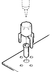
Even better, if feasible, is to design in dedicated high-frequency test points on the board (Figure 11). Such probe-tip adaptors provide all of the above-mentioned advantages for using naked probe tips, offering the ability to measure numerous points quickly and accurately.
Probe-Capacitance Effects
Probe capacitance affects rise time and amplitude measurements; it can also affect the stability of certain devices.
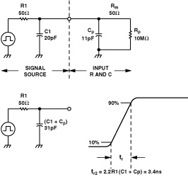
The probe capacitance adds directly to the node capacitance being probed. The added capacitance increases the node time constant, which slows down the rising and falling edges of a pulse. For example, if a pulse generator is connected to an arbitrary capacitive load, where CL = C1, as shown in Figure 12, then the associated rise time can be calculated from Equation 8, where RS (= R1, in Figure 12), is the source resistance.
 | (7) |
If RS = 50 ohms and CL = 20 pF, then tr = 2.2 ns.
Next, let’s consider the same circuit probed with a 10 pF, 10× probe. The new circuit is shown in Figure 13. The total capacitance is now 31 pF and the new rise time is 3.4 ns, a more than 54% increase in rise time! Clearly this isn’t acceptable, but what other choices are there?
Active probes are another good choice for probing high speed circuits. Active, or FET, probes contain an active transistor (typically an FET) that amplifies the signal, compared to passive probes that attenuate the signal. The advantage of active probes is their extremely wide bandwidth, high input impedance, and low input capacitance. Another alternative is to use a scope probe with a high attenuation factor. Typically, higher-attenuation-factor probes have less capacitance.
Not only can the probe tip capacitance cause errors in rise time measurements; it can also cause some circuits to ring, overshoot, or, in extreme cases, become unstable. For example, many high-speed operational amplifiers are sensitive to the effects of capacitive loading at their output and at their inverting input.
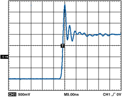
When capacitance (in this case, the scope probe tip) is introduced at the output of a high-speed amplifier, the amplifier’s output resistance and the capacitance form an additional pole in the feedback response. The pole introduces phase shift and lowers the amplifier’s phase margin, which can lead to instability. This loss of phase margin can cause ringing, overshoot, and oscillations. Figure 14 shows the output of a high-speed amplifier being probed with a Tektronix P61131 10 pF, 10× scope probe, using proper high-speed grounding. The signal has a 1300 mV overshoot with 12 ns of sustained ringing. Obviously, this is not the right probe for this application.
Fortunately, there are a few solutions to this problem. First, use a lower-capacitance probe. In Figure 15, a Tektronix P6204 1.1 GHz active 10× FET probe, with 1.7 pF, is used to make the same measurement as is shown in Figure 14, again with proper high-speed grounding.
In this case, there is significantly lower overshoot (600 mV) and ringing (5 ns) using the lower capacitance active probe.
Another technique is to include a small amount of series resistance, (typically 25 ohms to 50 ohms) with the scope probe. This will help isolate the capacitance from the amplifier output and will lessen the ringing and overshoot.
Propagation Delay
An easy way to measure propagation delay is to probe the device under test (DUT) at its input and output simultaneously. The propagation delay can be readily read from the scope display as the time difference between the two waveforms.
When measuring short propagation delays (<10 ns), however, care must be taken to ensure that both scope probes are the same length. Since the propagation delay in wire is approximately 1.5 ns/ft, sizeable errors can result from pairing probes of different lengths. For example, measuring a signal’s propagation delay using a 3 ft probe and a 6 ft probe can introduce approximately 4.5 ns of delay error—a significant error when making single- or double-digit nanosecond measurements.
If two probes of equal length are not available (often the case), do the following: Connect both probes to a common source (e.g., a pulse generator) and record the propagation delay difference. This is the “calibration factor.” Then correct the measurement by subtracting this number from the longer-probe reading.
CONCLUSION
While high-speed testing is not overly complicated, numerous factors must be considered when venturing into the lab to make high-speed time-domain measurements. Bandwidth, calibration, rise-time-measuring scope and probe selection, and probe-tip and ground-lead lengths all play important roles in the quality and integrity of measurements. Employing some of the techniques mentioned here will help speed up the measurement process and improve the overall quality of results. For more information, visit www.analog.com and www.tek.com.
参考电路
1 ABC’s of Probes Primer. Tektronix, Inc. 2005.
2 Mittermayer, Christoph and Andreas Steininger. “On the Determination of Dynamic Errors for Rise-Time Measurement with an Oscilloscope.” IEEE Transactions on Instrumentation and Measurement, 48-6. December 1999.
3 Millman, Jacob and Herbert Taub. Pulse, Digital, and Switching Waveforms. McGraw-Hill, 1965. ISBN 07-042386-5.
4 The Effect of Probe Input Capacitance on Measurement Accuracy. Tektronix, Inc. 1996.
致谢
Figures 1, 6, 7, 8, 11, 12, and 13 appear courtesy of Tektronix, Inc., with permission.


 客服微信
客服微信 查ic网订阅号